A Step-by-Step Guide to Create Google Sheets Heatmap

Nobody likes sifting through endless rows of data in a spreadsheet.  

Especially when analyzing crucial data to identify trends or patterns in visitor behavior impacting your business. 

Using heatmaps in Google Sheets solves this problem. It gives your data a simple yet powerful touch and helps you uncover important trends and actionable insights. 

So, let’s take a closer look at how you can effectively use heatmaps to convert boring data into interesting visuals with just a few clicks.

Does Google Sheets have a heatmap tool?

No, Google Sheets does not offer a typical heatmap tool. However, you can use the built-in ‘conditional formatting’ feature to create a heatmap. 

This method is quite straightforward and it also helps you to present your data in a more visually appealing way.   

Also, creating a heatmap with the help of conditional formatting allows you to quickly identify patterns, trends, or specific outliers in your data. 

What are the steps to create a heatmap in Google Sheets?

The process of creating a heatmap in Google Sheets is quite easy, especially if you are familiar with the tool. You can create a heatmap to represent any data set with values.  

For example, let’s consider that you wish to compare the region-wise performance of the key pages on your website. You’ve gathered the CTR data for each page in a Google Sheet and this is how it looks at first. 

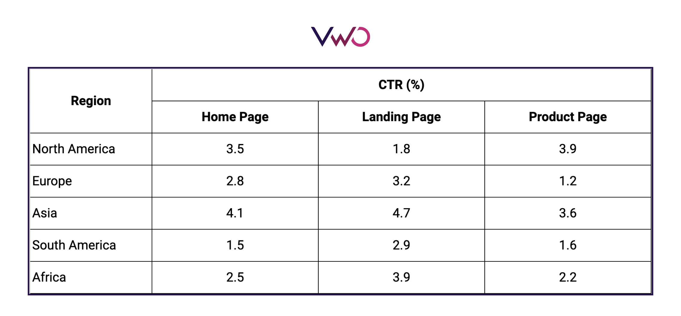
Here’s how you can create a heatmap to represent this kind of data set. 

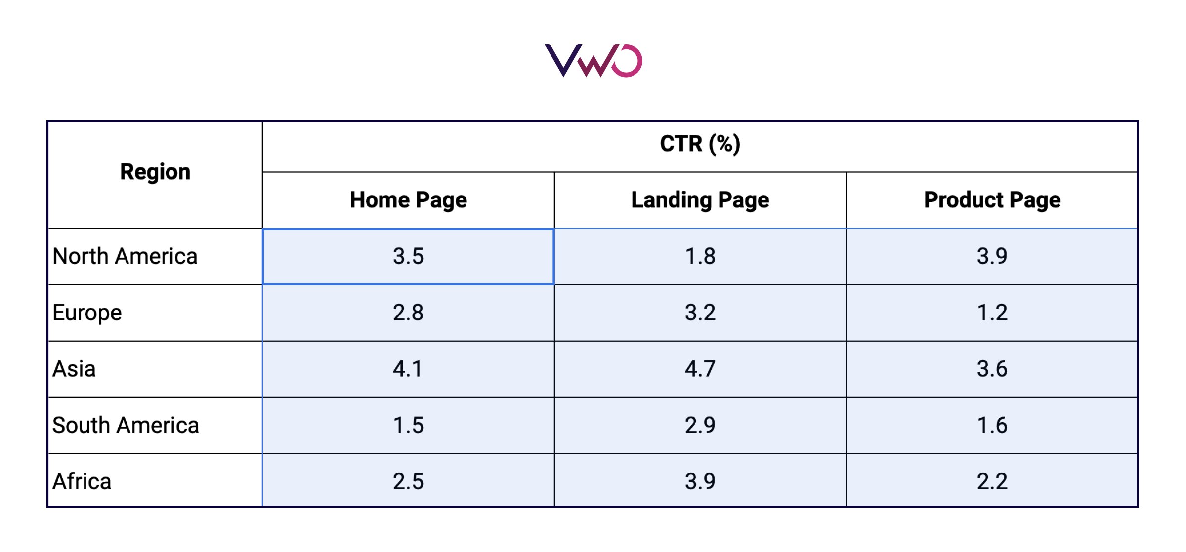
Step 1 – Select the data range

Select or highlight the cells that contain the data you want to analyze. In our example, we will select the data from cells B3 to D7. Make sure you avoid selecting the titles or category headings.

Step 2 – Click on ‘Format > Conditional formatting’

Once, you’ve selected the data range, go to the menu bar at the top and click on Format. Select Conditional formatting and a new tab will appear on your screen.

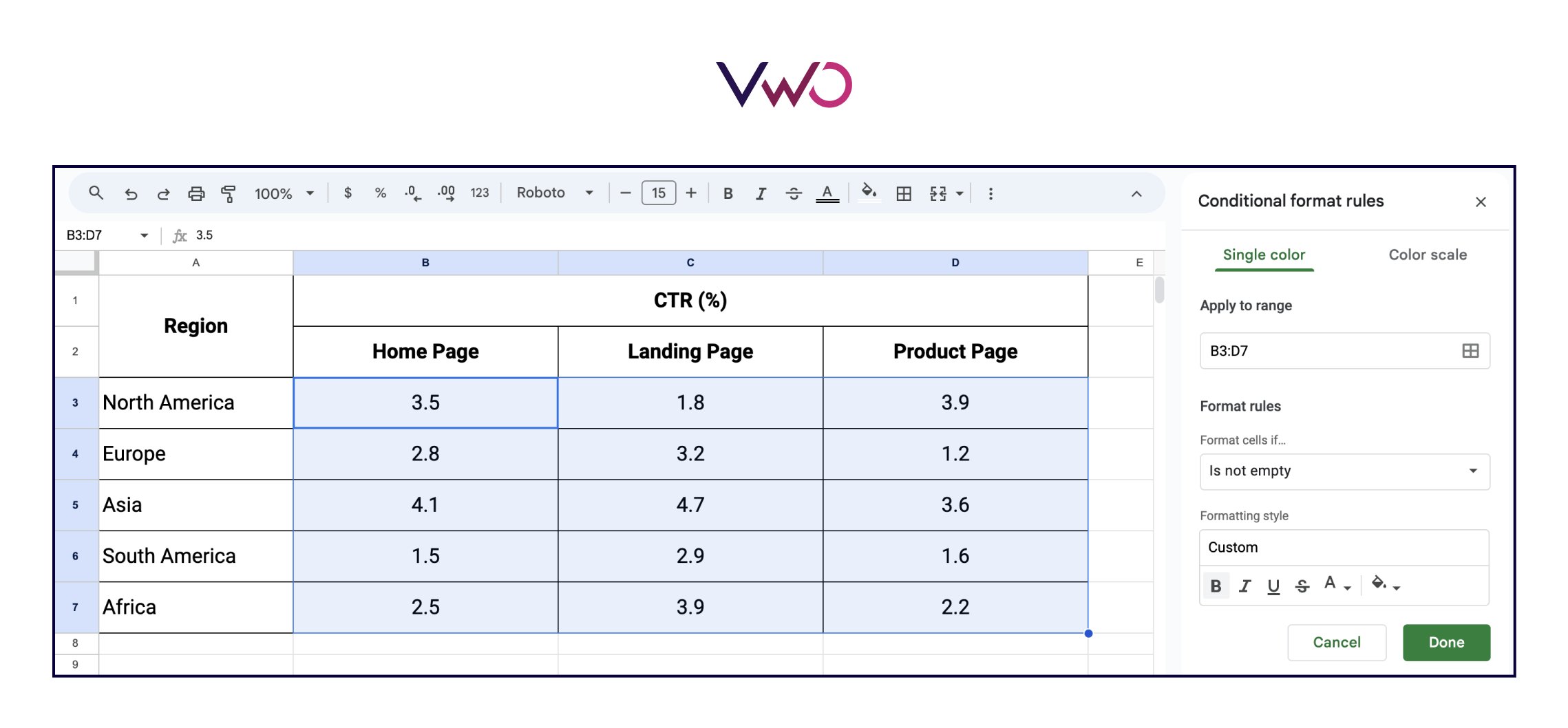
Step 3 – Go to ‘Color scale’ and click on ‘Format rules’

Here, click on the ‘Color scale’ section to set the rules for your heatmap. Google Sheets offers a set of default color scales that you can choose from the ‘Format rules’ tab. 

Additionally, you can modify the rules and customize the heatmap according to your requirements. For instance, in the ‘Format rules’ tab, click on the Custom color scale option.

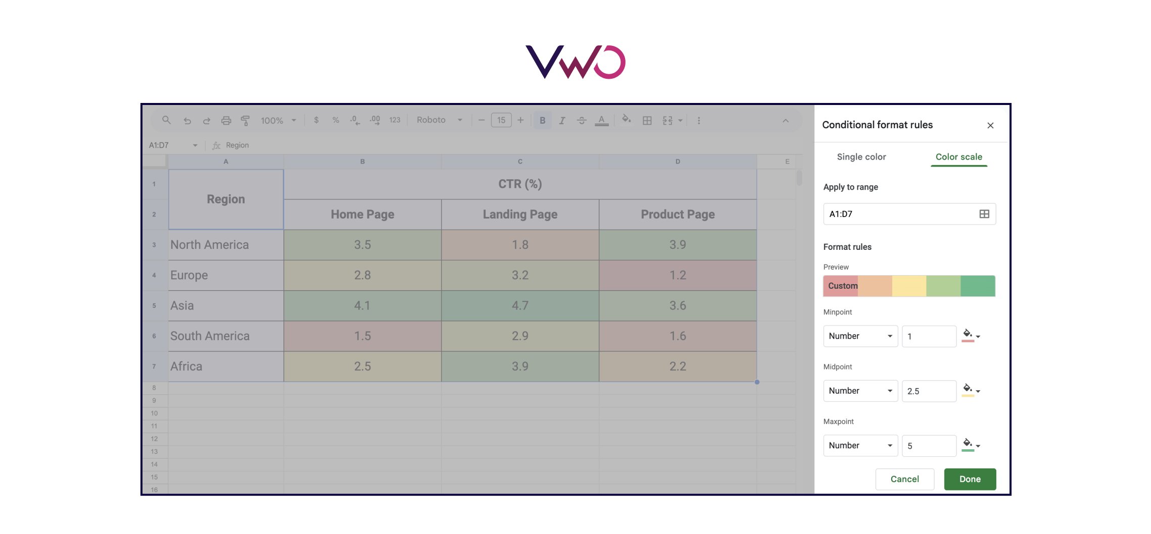
Now, you can set the rules for your heatmap by entering different high and low values for the Minpoint, Midpoint, and Maxpoint. Based on our example, we will set it as:

Minpoint CTR – 1

Midpoint CTR – 2.5

Maxpoint CTR – 5

Step 4 – Review the rules and apply formatting

Once you’ve configured the data values for each category, click Done. You’ve successfully created a Google Sheets heatmap and you can now analyze the region-wise CTR data for different pages.

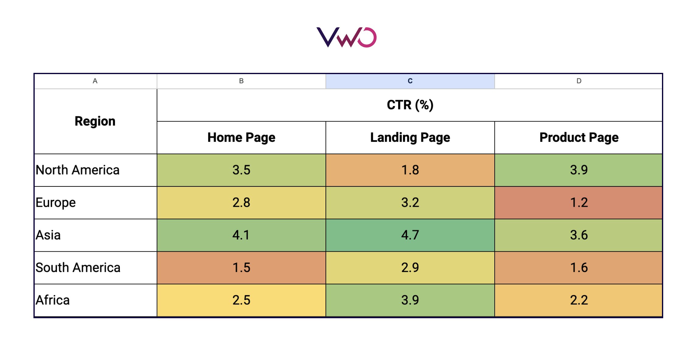
From the heatmap data, you can easily identify the specific regions and pages that need optimization. 

For instance, the home page visible for the South American audience has quite a low CTR as compared to other regions. Similarly, European visitors are not engaging enough with the product page.

Based on this data, you can take necessary actions to improve the performance of these pages.

Moreover, you can further modify the rules and choose different color gradients to create a more customized heatmap in Google Sheets.   

Examples and real-world applications of heatmaps in Google Sheets

Now that we’ve covered the process of creating heatmaps, here are some practical examples of how you can use them to analyze data in different contexts.

1. Analyze website performance

Suppose you manage a website and want to understand which pages are attracting the most visitors and which ones are underperforming. 

You can create a heatmap to visualize page views across different sections of your site. By applying a color scale, you can quickly identify high-traffic pages (highlighted in green) and low-traffic pages (highlighted in red). 

This helps in making data-driven decisions, like optimizing content on underperforming pages or promoting high-traffic ones further.

2. Analyze sales performance

For businesses operating in multiple regions, a heatmap can offer a clear view of sales performance across different areas. 

Let’s say you’ve collected quarterly sales data from different regions. A heatmap allows you to spot which regions are excelling and which are lagging. This type of data visualization helps in directing resources and efforts to regions that need improvement.

3. Compare test scores

Teachers can use heatmaps to analyze student performance across different subjects. 

By inputting test scores into Google Sheets and applying a heatmap, a teacher can easily see which students excel in certain subjects and which ones may need extra help. 

For instance, scores in the 90-100% range could be highlighted in green, while those below 60% might be shown in red. This allows teachers to quickly identify patterns and address any learning gaps.

4. Track project-related tasks

In a project management scenario, a heatmap can be used to monitor the status of various tasks. 

Let’s say you’re tracking the completion percentage of tasks across multiple projects. A heatmap can visually indicate which tasks are on track (green), which are at risk (yellow), and which are behind schedule (red). 

This makes it easier to prioritize tasks that require immediate attention, ensuring that projects stay on schedule.

How to create better heatmaps in Google Sheets?

While creating a heatmap, you must also ensure that your data is organized in a way that makes it easy to apply and interpret. Here are some tips to get started.

Structure your data

Whether it is for website analytics or any other use case, your data must be organized in a clear and consistent format. Typically, you’ll have one column for categories (e.g., regions, products, or dates) and another for the corresponding key data points you want to visualize (e.g., sales figures, page views, or conversion rates).

Clean your data

Make sure your data is free from errors or inconsistencies, such as missing values or outliers, that could skew your heatmap. Removing any irrelevant points will ensure that your heatmap provides an accurate representation of your data.

Decide on the range

Identify the range of data you want to include in your heatmap. This might be a single column or multiple columns of data, depending on what you want to visualize.

By carefully preparing your data, customizing color scales, and understanding how to interpret the results, you can identify patterns, observe trends, and gather deeper insights into your data. 

Heatmaps by VWO Insights – Web  

If you are looking for a more comprehensive way to visualize visitor journeys on your website, you can use the Heatmaps feature offered as part of VWO Insights – Web.

The platform offers a wide variety of heatmap types such as dynamic heatmaps, clickmaps, scrollmaps, etc. You can use these heatmaps to observe how visitors interact with your website and analyze their behavior in a more nuanced way. 

Take a free trial of VWO Insights – Web to explore heatmaps, session recordings, and many other exciting features to analyze visitor behavior on your website. 

Frequently asked questions