(This post is a scientific explanation of the optimal sample size for your tests to hold true statistically. VWO’s test reporting is engineered in a way that you would not waste your time looking up p-values or determining statistical significance – the platform reports ‘probability to win’ and makes test results easy to interpret. Sign up for a free trial here)
How large does the sample size need to be?
In the online world, the possibilities for A/B testing just about anything are immense. And many experiments are done indeed, the result of which are interpreted following the rules of null-hypothesis testing, “are the results statistically significant?”
An important aspect in the work of the database analyst then is to determine appropriate sample sizes for these tests.
Download Free: A/B Testing Guide
On the basis of a daily case, a number of current approaches for calculating desired sample size are discussed.
Case for calculating sample size
The marketer has devised an alternative for a landing page and wants to put this alternative to a test. The original landing page has a known conversion of 4%. The expected conversion of the alternative page is 5%. So the marketer asks the analyst “how large should the sample be to demonstrate with statistical significance that the alternative is better than the original?”
Solution: “default sample size”
The analyst says: split run (A/B test) with 5,000 observations each and a one-sided test with a reliability of .95. Out of habit.
What happens here?
What happens when drawing two samples to estimate the difference between the two, with a one-sided test and a reliability of .95? This can be demonstrated by infinitely drawing two samples of 5,000 observations neach from a population with a conversion of 4%, and plotting the difference in conversion per pair (per ‘test’) between the two samples in a chart.
Figure 1: sampling distribution for the difference between two proportions with p1=p2=.04 and n1=n2=5,000; a significance area is indicated for alpha=.05 (reliability= .95) using a one-sided test.
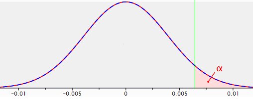
This chart reflects what is formally called the ‘sampling distribution for the difference between two proportions.’ It is the probability distribution of all possible sample results calculated for the difference between p1=p2=.04 andn1=n2=5,000. This distribution is the basis –the reference distribution- for null hypothesis testing. The null hypothesis being that there is no difference between the two landing pages. This is the distribution used for actually deciding on significance or non-significance.
p=.04 means 4% conversion. Statisticians usually talk about proportions that can lie between 0 and 1, whereas in the everyday language mostly percentages are communicated. In order to comply with the chart, the proportion notation is used.
This probability distribution can be replicated roughly using this spss syntax (thirty paired samples from a population.sps). Not infinitely, but 30 times two samples are drawn with p1=p2=.04 and n1=n2=5,000. The difference between the two samples are then plotted in a histogram with the normal distribution inputted (the last chart in the output). This normal curve will be quite similar to the curve in figure 1. The reason for performing this experiment is to demonstrate the essence of a sampling distribution.
The modal value of the difference in conversion between the two groups is zero. That makes sense, both groups come from the same population with a conversion of 4%. Deviations from zero both to the left (original does better) and to the right (alternative does better) can and will occur, just by chance. The further from zero, however, the smaller the probability of happening. The pink area with the character alpha indicated in it is the significance area, or unreliability=1-reliability=1-.95.
If in a test the difference in conversion between the alternative page and the original page falls in the pink area, then the null hypothesis that there is no difference between both pages is rejected in favour of the hypothesis that the alternative page returns a higher conversion than the original. The logic behind this is that if the null hypothesis were really true, such result would be a rather ‘rare’ outcome.
The x axis in figure 1 doesn’t display the value of the test statistic (Z in this case) as would usually be the case. For clarity sake the concrete difference in conversion between the two landing pages has been displayed.
So when in a split run test the alternative landing page returns a conversion rate that is 0.645% higher or more than the original landing page (hence falls in the significance area), then the null hypothesis stating there is no difference in conversion between the landing pages is rejected in favour of the hypothesis that the alternative does better (the 0.645% corresponds to a test statistic Z value of 1.65).
Advantage of the approach “default sample size” is that by choosing a fixed sample size, a certain standardization is brought in. Various tests are comparable ‘stand an equal chance’ to that respect.
Disadvantage to this approach is that whereas the chance to reject the null hypothesis when the null hypothesis (H0) is true is well known, namely the self-selected alpha of.05, the chance to not reject H0when H0 is not true remains unknown. These are two false decisions, known as type 1 error and type 2 error respectively.
A type 1 error, or alpha, is made when H0 is rejected, when in fact H0 is true. Alpha is the probability of saying on the outcome of a test there is an effect for the manipulation, while on population level there actually is none. 1-alpha is the chance to accept the null hypothesis when it is true –a correct decision-. This is called reliability.
A type 2 error, or beta, is made when H0 is not rejected, when in fact H0 is not true. Beta is the probability of saying on the outcome of a test there is no effect for the manipulation, while on population level there actually is. 1-beta is the chance to reject the null hypothesis when it is not true–a correct decision-. This is called power.
Power is a function of alpha, sample size and effect (the effect here is the difference in conversion between the two landing pages, i.e. at population level the added value of the alternate site compared to the original site). The smaller alpha, sample size or effect the smaller power is.
In this example alpha is set by the analyst at.05. Sample sizes are also set by the analyst, 5000 for original, 5000 for alternative. Which leaves the effect. And the actual effect is by definition unknown. However it is not unrealistic to use commercial targets or experiential numbers as an anchor value, as was formulated by the marketer in the current case: an expected improvement from 4% to 5%. Now if that effect were really true, the marketer of course would want to find statistically significant results in a test.
An example may help to make this concept insightful and to clarify the importance of power: suppose the actual (=population) conversion of the alternative page is indeed 5%. The sampling distribution for the difference between two proportions with conversion1=4%, conversion2=5% and n1=n2=5,000is plotted in combination with the previously shown sampling distribution for the difference between two proportions with conversion1=conversion2=4% and n1=n2=5,000 (figure 1).
Figure 2: sampling distributions for the difference between two proportions with p1=p2=.04, n1=n2=5,000(red line) and p1=.04, p2=.05, n1=n2=5,000 (dotted blue line), with a one-sided test and a reliability of .95.
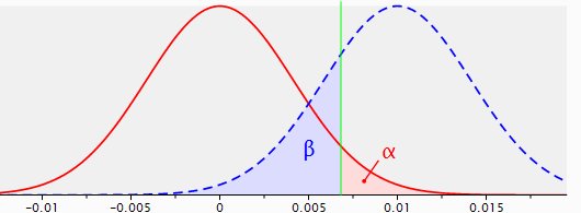
The dotted blue line shows the sampling distribution of the difference in conversion rates between original and alternative when in reality (on population level) the original page makes 4% conversion and the alternate page 5%, with samples of 5,000 each. The sampling distribution whenH0 is true, the red line, has basically shifted to the right. The modal value of this new distribution with the supposed effect of 1% is of course 1%, with random deviations both tothe left and to the right.
Now, all outcomes, i.e. test results, on the right side of the green line (marking the significance area) are regarded as significant. All observations on the left side of the green line are regarded as not significant. The area under the ‘blue’ distribution left of the significance line is beta, the chance to not reject H0 when H0is in fact not true (a false decision), and it covers 22% of that distribution.
That makes the area under the blue distribution to the right of the significance line the power area and this area covers 78% of the sampling distribution. The probability to reject H0 when H0is not true, a correct decision.
So the power of this specific test with its specific parameters is .78.
In 78% of the cases when this test is done, it will yield a significant effect and consequent rejecting of H0. Could be acceptable, or could perhaps not be acceptable; that is a question for marketer and analyst to agree upon.
No simple matter, but important. Suppose for example that an expectation of 10% increase in conversion would be realistic as well as commercially interesting: 4.0% original versus 4.4% for the alternative. Then the situation changes as follows.
Figure 3: sampling distributions for the difference between two proportions with p1=p2=.040, n1=n2=5,000 (red line) and p1=.040, p2=.044, n1=n2=5,000 (dotted blue line), with a one-sided test and a reliability of .95.
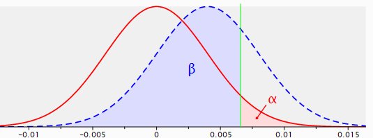
Now the power is.26. Under these circumstances the test would not make much sense, is in fact counter-productive, since the chance that such test will lead to a significant result is as low as .26.
The above figures are calculated and made with the application ‘Gpower’:
This program calculates achieved power for many types of tests, based on desired sample size, alpha, and supposed effect.
Likewise required sample size can be calculated from desired power, alpha and expected effect, required alpha can be calculated from desired power, sample size and expected effect and required effect can be calculated from desired power, alpha and sample size.
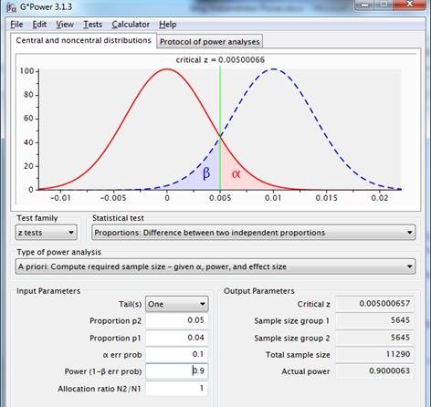
Should a power of .95 be desired for a supposed p1=.040, p2=.044, then the required sample sizes are 54.428 each.
Figure 4: sampling distributions for the difference between two proportions with p1=p2=.040 (red line) and p1=.040, p2=.044 (dotted blue line), using a one-sided test, with a reliability of .95 and a power of .95.
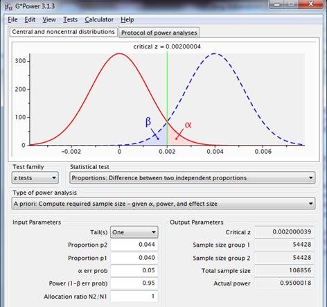
This figure shows information omitted in previous charts. This also gives an impression of the interface of the program.
Download Free: A/B Testing Guide
Important aspects of power analysis are careful evaluation of the consequences of rejecting the null hypothesis when the null hypothesis is in fact true – e.g. based on test results a costly campaign is implemented under the assumption that it will be a success and that success doesn’t come true – and the consequences of not rejecting the null hypothesis when the null hypothesis is not true -e.g. based on test results a campaign is not implemented, whereas it would have been a success.
Solution: “default number of conversions”
The analyst says: split run with a minimum of 100 conversions per competing page and a one-sided test with a reliability of .95.
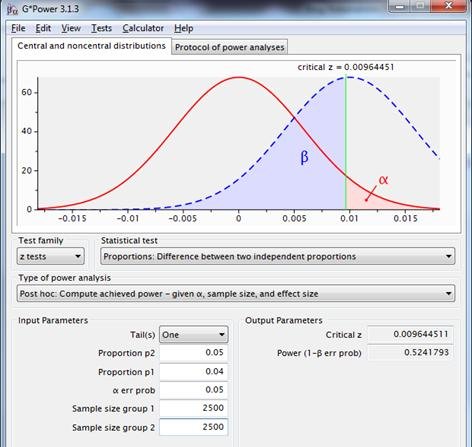
In the current case with expected conversion of the original page 4% and expected conversion of the alternate page 5%, a minimum of 2,500 observations per page will be advised.
When put to the power test though, this scenario demonstrates a power of just little over .5.
Figure 5: sampling distributions for the difference between two proportions with p1=p2=.04, n1=n2=2500 (red line) and p1=.04, p2=.05, n1=n2=2500 (dotted blue line) rusing a one-sided test, with a reliability of .95.
For a better power, a greater effect should be present, a larger sample size must be chosen, or alpha should be increased, e.g. to .2:
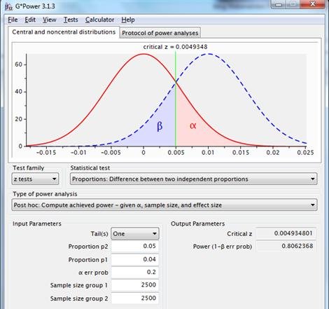
An alpha of .2 returns a power of .8. The power is more acceptable; the ‘cost ‘ for this bigger power consists of a magnified chance to reject H0 when H0 is actually true.
Again, business considerations involving the impact of alpha and beta play a key role in such decisions.
Approach “default number of conversions” with its rule of thumb on the number of conversions actually puts a kind of limit on effect sizes that still make sense to be put to a test (i.e. with a reasonable power). In that regard it also comprises a sort of standardization and that in itself is not a problem, as long as its consequences are understood and recognized.
Solution: “significant sample result”
The analyst says: split run with enough observations to get a statistical significant result if in the test the supposed effect and actually occurs, tested one-sided with a reliability of .95.
That sounds a little weird, and it is. Unfortunately this logic is often applied in practice. The required sample size is basically calculated assuming the supposed effect to actually occur in the sample.
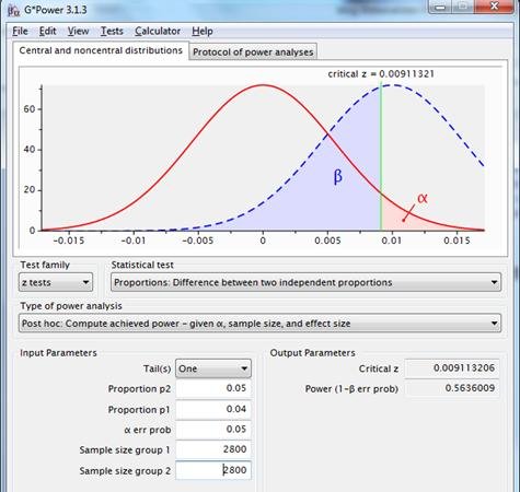
In the used example: if in a test the original has a conversion of 4% and he alternative 5%, then 2,800 cases per group would be necessary to reach statistical significance. This can be demonstrated with the accompanying spss syntax (limit at significant test result.sps).
These sort of calculations are applied by various online tools offering to calculate sample size. This approach ignores the concept of random sampling error, thus ignoring the essence of inferential statistics and null hypothesis testing. In practice, this will always yield a power of .5 plus a small additional excess.
Figure7: sampling distributions for the difference between two proportions with p1=p2=.04, n1=n2=2800 (red line) and p1=.04, p2=.05, n1=n2=2800 (dotted blue line), using a one-sided test, with a reliability of .95.
Using this system a sort of standardisation is actually also applied, namely on power, but that’s not the apparent goal this method was invented for.
Solution: “default reliability and power”
The analyst says: split run with a power of .8 and a reliability of .95 with a one-sided test.
In the current case with 4% conversion for original page versus 5% expected conversion for the alternate page, alpha=.05 and power=.80, Gpower advises two samples of 5313.
Figure 8: sampling distributions for the difference between two proportions with p1=p2=.04(red line) and p1=.04, p2=.05 (dotted blue line), using a one-sided test with reliability .95 and power .80.
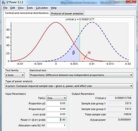
This approach uses desired reliability, expected effect and desired power in the calculation of the required sample size.
Now the analyst has grip on the probability an expected/desired/necessary effect will lead to statistically significant results in a test, namely .8.
Some online tools, for example VWO’s Split Test Duration Calculator, use the concept of power in their sample size calculation.
In a presentation by VWO “Visitors needed for A/B testing” a power of .8 is mentioned as a regular measure.
It can be questioned why that should be an acceptable rule? Why could the size of the power, as well as the size of the reliability not be used more dynamically?
Solution: “desired reliability and power”
The analyst says: split run with desired power and reliability using a one-sided test.
Follows a discussion on what is acceptable power and reliability in this case, with as a conclusion, say, both 90%. Result according to Gpower, 2 times 5.645 observations:
Figure 9: sampling distributions for the difference between two proportions with p1=p2=.04 (red line) and p1=.04, p2=.05 (dotted blue line), using a one-sided test with reliability=.90 and power=.90.
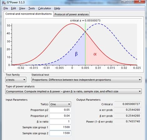
What if the marketer says “It takes too long to gather that many observations. The landing page will then not be important anymore. There is room for a total of 3,000 test observations. Reliability is equally important as power. The test should preferably be carried out and a decision should follow”?
Result on the basis of this constraint: reliability and power both .75. If this doesn’t pose problems for those concerned, the test may continue on the basis of alpha=.25 and power=.75.
Figure 10: sampling distributions for the difference between two proportions with p1=p2=.04, n1=n2=1500 (red line), and p1=.04, p2=.05, n1=n2=1500(dotted blue line), using a one-sided test with equal reliability and power.
This approach allows for flexible choice of reliability and power. The consequent lack of standardization is a disadvantage.
Conclusion
There are multiple approaches to calculate the required sample size, from questionable logic to strongly substantiated.
For strategically important ‘crucial experiments’, preference goes out to the most comprehensive method in which both “desired reliability and power” are involved in the calculation. If there is no possibility of checking against prior effects, an effect can be estimated using a pilot with “default sample size” or “default number of conversions”.
For the majority of decisions throughout the year “default reliability and power” is recommended, for reasons of comparability between tests.
Working with the recommended approaches based on calculated risk will lead to valuable optimization and correct decision making.
Note: Screenshots used in the blog belong to the author.
FAQs on A/B testing sample size
There are multiple approaches to determine the required sample size for A/B testing. For strategically important ‘crucial experiments’, preference goes out to the most comprehensive method in which both “desired reliability and power” are involved in the calculation.
In the online world the possibilities for a/b testing just about anything are immense. The sample size should be large enough to demonstrate with statistical significance that the alternative version is better than the original.
Categories: