The Relationship Behind Statistical Significance

A logician and a statistician were walking through a forest when they came across a river. A safety sign near the river said – the river is 4 feet deep on average. The logician reasoned that he is about 6 feet tall, and hence should be able to cross the river with ease. The logician walked in and drowned, while the statistician returned. Why did the statistician choose not to cross the river?

When faced with randomness, the immediate instinct of most is to ask for what happens on average. However, the statistician knows that the average can often be a convenient answer to hide the truth. The truth about how good or how bad things can be on the extreme. Some metrics deviate only slightly around the average, whereas others show big deviations on both sides that render the average meaningless. The statistician chose not to cross the river because it could have been very shallow in some places and very deep in others, still being 4 feet deep on average.

Most statistical methods hence take into consideration the standard deviation which has come to be the accepted measure for the spread of data. If the standard deviation is high, the data is widely spread. If the standard deviation is low, the data is tightly bound around the average. The average represents the central tendency of the metric if all the randomness were to be stripped apart. The standard deviation represents the chaos that renders the randomness in the first place.

The standard deviation plays a pivotal role in determining the statistical significance as it acts as the yardstick to compare the effect-size against. While the previous post explained the three forces behind statistical significance, this post will intuitively explain the relationship between these three forces. All that statistical significance is can be broken down into the following relationship:

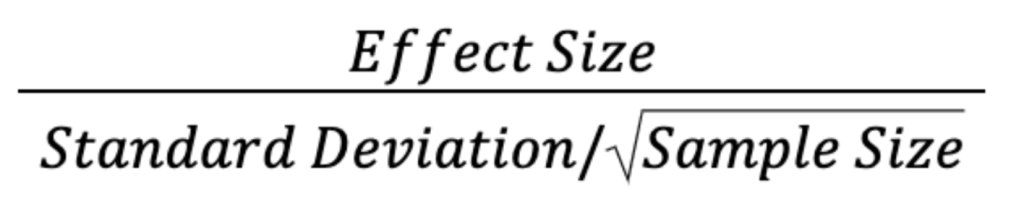
To build an intuition of the relationship above, we need to break it down into two parts and explore it piece by piece.

Effect Size – Standard Deviation Ratio

Let us start by reminding ourselves that the purpose of statistical significance is to tell us if the observed difference between two groups is statistically significant or not. In other words, is the difference larger than what you would expect purely by chance?

It is worth noting here that any two groups of random samples can never show exactly the same average (assuming the group is large enough). So, whenever you calculate the average of the two groups, there will be some difference between the two averages. The question is if this difference is large enough. Answering this question, demands a yard-stick to compare the difference. This yard-stick is the standard deviation.

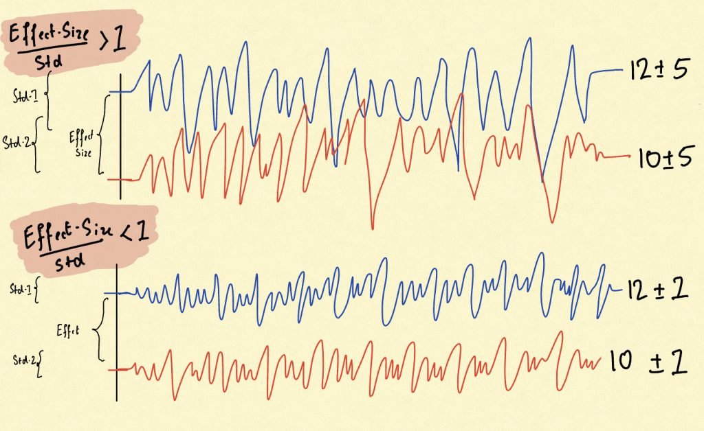
For understanding, observe the sketch above. The blue signal represents the variation and the red signal represents the control. There are two cases shown. Both have the same average value of control and variation (10 and 12 respectively) and the same average difference as well (2). However, the upper one has a much greater standard deviation of 5, whereas the lower one has a lesser standard deviation of 1. Now visually zoom out and judge, which of the two signals seem well separated.

Note that even when the averages are the same, the one with the lower standard deviation seems to be well separated and hence the effect size of 2 seems more statistically significant in the second case. The ratio between the effect-size and the standard deviation is the fundamental determinant behind statistical significance. As this ratio rises, the effect-size becomes more statistically significant. As this ratio falls, the effect-size becomes less statistically significant.

But wait, where does sample size fit in?

The Standard Deviation of the Mean

To understand the role of sample sizes in statistical significance, we need to first understand the difference between the standard deviation of the samples and the standard deviation of the mean. Note that while measuring statistical significance, we essentially intend to compare the means of the two populations and not exactly the samples. Statistical significance aims to calculate the chance that the two groups behave differently ‘on average’. 

To understand further, suppose you are running an A/B test and want to test if the variant improves the revenue per sale on your website. Note that every visitor will give some revenue on your website. You do not intend to improve the revenue given by every visitor, you only intend to improve the revenue per sale on average. This means that if a visitor on average gives a 5$ revenue on control, and 5.1$ on variation, you will still consider the variation to be a winner. This may include many visitors on variation who give a lesser revenue than many visitors on control. But what matters is that on average the variation performed better.

Note that the standard deviation we understand is that of the samples. So, if the revenue samples vary between 3$ – 7$, it represents the spread of the samples and not that of the mean.

In the effect-size vs standard deviation ratio, what should come in the denominator is not the standard deviation of the samples but rather that of the mean. Calculating the standard deviation of the samples is straightforward, but to calculate the standard deviation of the mean, we need to understand the perspective of sampling theory.

The Population Mean and The Sample Mean

Sampling Theory is an integral part of statistics because to resolve randomness in any process, a statistician first needs a sample to work with. Sampling Theory starts by first differentiating the sample from the population. The population is the entire set of entities that you are concerned with. For instance, in the case of an A/B test, this population is the set of all the visitors that your website will ever have.

However, you can only observe a sample, and never the entire population. But on the contrary, what you are really interested in is the population mean which is latent and unobservable. What you get is the sample mean which will change slightly every time you collect a random sample.

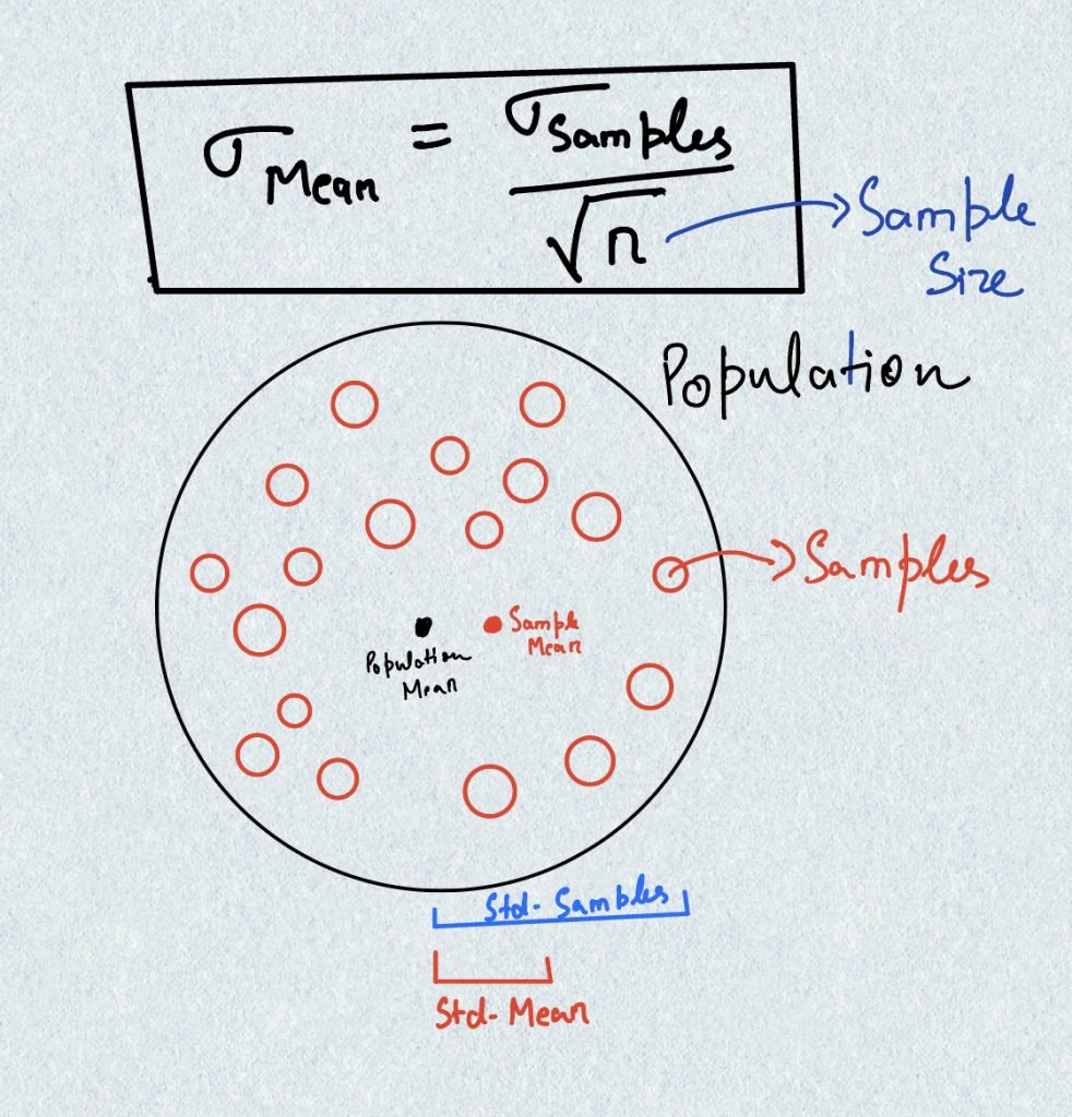
Sampling Theory gives us the relationship between the population mean and the sample mean. Let us imagine a flat 2-dimensional pie that represents the entire population. Let us also assume that the center of the pie represents the population mean and the width of the pie represents the spread of the data. So, if the metric of interest is widely spread around the mean, the wider will be the pie. Hence, the width of the pie corresponds to the standard deviation of the samples.

Now suppose you collect a sample on the pie, which is sort of like some randomly placed blueberries on the surface. These blueberries are the samples whose positions are known. You now calculate the center of all these blueberries which is the sample mean. The question is, how far is the center of the blueberries (the sample mean) from the center of the pie (the population mean)? (Observe the sketch drawn above).

Sampling Theory tells us that the difference between the sample mean and the population mean depends on two things: Firstly, the overall width of the pie (the standard deviation of the samples) and the secondly, the number of blueberries (the sample size).

The difference between the sample mean and the population mean is the standard deviation of the mean and is also called the standard error. Since, the population mean in reality is unobservable, the standard error reports the uncertainty in the sample mean. The exact formula can be observed in the sketch drawn.

If you substitute the standard deviation of the mean in the effect-size vs standard deviation ratio, you see that the formula given in the introduction emerges. Take a minute to observe how both ideas come together to define statistical significance.

Conclusion

There are various procedures in statistics for determining statistical significance in different contexts. However, the core intuition of all procedures boils down to the same three factors in different contexts. A very interesting debate in statistics is that of the Frequentists and the Bayesians and how they calculate statistical significance using their own assumptions. Frequentist and Bayesian are two ways of looking at the same thing and in practice rely on the same relationship that has been explained in this post.

However, both perspectives are interesting in their own right and the difference between them is critical once you understand it. Bayesians introduce a fourth variable in statistical significance, the prior. The prior is something that is neither easy to estimate nor easy to refute but as we will see it does matter depending on how philosophically you choose to see the world.

In the upcoming posts, we will carry the exploration forward with this fourth variable and then dive deep into the debate between the Frequentists and the Bayesians.