The Fourth Factor in Statistical Significance

Let me take you through an interesting statistical puzzle. Suppose that there is a rare disease that infects 1 in 1000 people and scientists develop a test that has a 5% false positive rate. This means that the disease will be detected for sure if the patient is infected, but the test will also detect the disease with a 5% chance if the patient is not infected. The question is if you test positive for this disease, what is the chance that you are actually infected? The answer is 2%.

So, let us break this down. If 1000 people get tested for this disease, there will be 1 truly infected person who will be detected as positive. Also, there will be 999 uninfected people, out of which almost 50 will be detected as positive due to the 5% false positive rate. So, 51 people in total will be detected as positive but only 1 of them will actually be infected. 1/51 comes out to be roughly 2% which is the chance that you have the disease after you have been tested as positive by a fairly accurate testing mechanism.

Most readers who are not well-versed in Bayesian statistical thinking will tend to find this result odd. But you can try sitting with this for a while and you will realize that the result is statistically sound. This is just how statistics work. It looks odd to us because it goes against our intuition. The key factor in the above problem that is creating the counter-intuition is the extremely low prevalence of the disease in the population.

This is the fourth factor that affects all tests of statistical judgment. It is fundamentally different from the other three forces of statistical significance, is highly counterintuitive to our understanding of probability, and is the cornerstone to understanding a distinct statistical ideology called the Bayesian statistics. In this post, I will explain this fourth factor and how it comes into play. To build intuition, I will use the context of testing for a disease. However, the ideas presented below apply to all statistical tests including the test of significance in experimentation.

Breaking down Statistical Accuracy

At the very base, a statistical testing procedure is designed for two kinds of inputs: The subjects that are positive (have the disease) and the subjects that are negative (do not have the disease). A testing procedure usually starts by defining a statistic that is used to decide if the subject is positive or negative. In the case of a disease, this can be some observable property of the patient’s body. Advanced tests will use a statistic derived from multiple parameters, but still they will be finally reduced to one number called the test statistic. 

Note that the underlying truth being tested is absolute, it is either positive or negative but not both. But it is hidden and what is observable is only the test statistic which is correlated to the truth but not an absolute representation. Hence, the test statistic is distributed over a range of values for the two types of subjects. The chosen test statistic is effective only if it separates the positives and negatives into two lumps. Ideally, the distribution of the test statistic should be something like the following: 

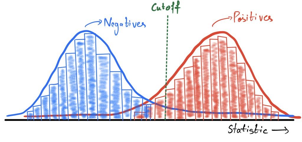
The statistical test has to define a cutoff which will be used to predict if the subject is positive or negative. This cutoff gives rise to two forms of statistical accuracy that are common to all testing procedures.

1. Accuracy for the positive subjects: The positive subjects are divided into two groups by the cutoff. These are the true positives (above the cutoff) and the false negatives (below the cutoff). Together the true positive rate and the false negative rate sum up to 1.

2. Accuracy for the negative subjects: The negative subjects are also divided into two groups. These are the true negatives (below the cutoff) and the false positives (above the cutoff). Similarly, the true negative rate and the false positive rate sum up to 1.

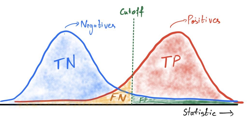
This is the conventional approach for studying the accuracy of any statistical test. False Positives and False Negatives are also known as Type-1 and Type-2 errors in hypothesis testing. Reporting one of the measures from each category defines the accuracy of the testing mechanism.

A More Relevant Question for Accuracy

However, if you look at things from a different lens there is a very relevant question of accuracy that gets missed out in the conventional approach. Observe the two questions below and think about how they are different. 

1. What is the chance that the patient is detected as positive if he actually has the disease? 

2. What is the chance that a patient has the disease if he has been detected as positive?

Note that while the answers to the two questions look similar, the answers can be drastically different. Let us first decipher what the second question asks for and how it is different from the first. Observe the image below.

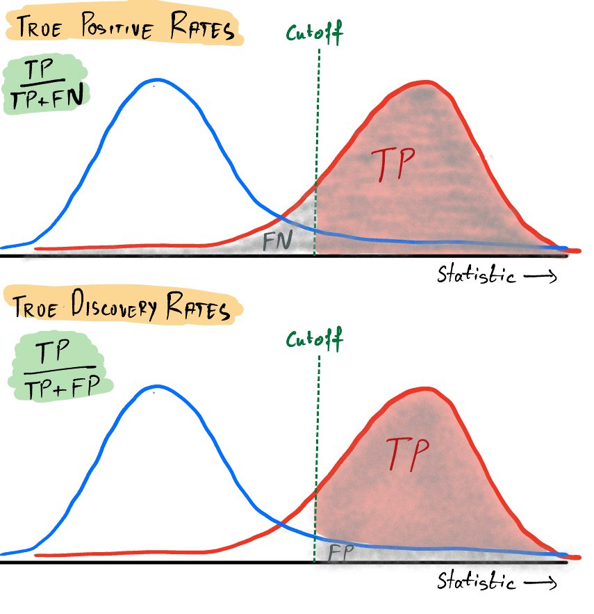
The first question asks how many of the red cases fall above the cutoff. On the other hand, the second question asks how many of the cases that fall above the cutoff are actually positive (red). It is known as the True Discovery Rate. 

The True Discovery Rate can be drastically different from the True Positive Rate depending on how many red items are there in the population. If the mix is densely populated with blue items, the true discovery rates are low. If the mix is densely populated with red items, the true discovery rates are high. The figure below shows what happens when we change the proportion of the red and blue items in the population.

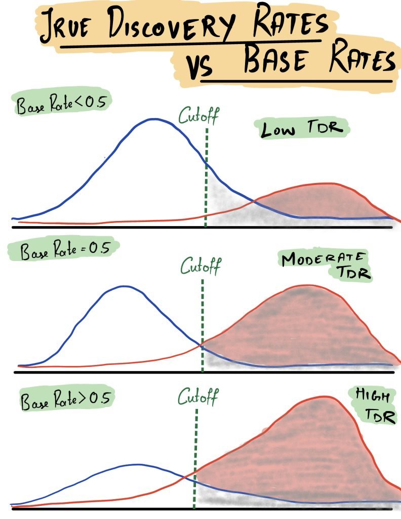
The proportion of this mix can be referred to by different names, one of them being the base rate of the phenomenon being tested. Base Rates are essentially the proportion of positives in the total population. They do not matter to the conventional measures of accuracy by design, but they matter a lot to the second type of question. The second type of question is more relevant in practice because you do not know in advance which subjects are positive and which subjects are negative.

Base Rates are the fourth factor in the determination of statistical significance but they get overlooked because they are very hard to measure. In future posts, we will discuss more on base rates and their implications on statistics and experimentation.

Conclusion

Base Rates form the fundamental difference between two distinct schools of thought in statistics, the Frequentists and the Bayesians. Frequentists have deep philosophical problems with the base rates because the base rates can never be empirically tested. In other words, there is no way to test if a chosen base rate is correct or not. Bayesians are more fond of addressing the second type of questions rather than the first. Bayesians hence have to define a prior that in practice refers to the base rates. But priors have often been misinterpreted and if defined wrongly, they bias the results. The debate between the Frequentists and the Bayesians has gone on ever since and we will explore it further in future posts.