The Bayesian Way To Statistical Significance

In the 1950s, the chess community needed a chess rating system to rank and match players with competent opponents. The United States Chess Federation used a system of rating players developed by a chess tournament organizer, Kenneth Harkness. However, the Harkness system was often found to be inaccurate because the ratings were adjusted by a static margin based on the outcome of a game. In essence, it meant that it did not matter whether you win against a weaker player or you win against a stronger player, a fixed number of points will be added to your rating. This obviously motivated chess players to play against weaker players and avoid playing against stronger ones. 

Arpad Elo, a Hungarian-American physics professor and skilled chess master identified this shortcoming and developed a new rating system. The new rating system differed from its predecessor because it made dynamic adjustments based on the difference in the existing rating of the two players. So, if a high-rated player lost against a low-rated player, the adjustment made would be larger compared to when a low-rated player lost against a high-rated player. From an epistemological perspective, Elo developed a way to include prior knowledge (base rates) of player skill into the inference derived from a chess match.

In a wider context, the same problem is faced in rating a player in all multiplayer games as well. The result of the game needs to be inferred in the context of your prior expectations. The Harkness system was inaccurate because it only relied on the outcome of the match (evidence), whereas the Elo system incorporated both the prior and the evidence. At the heart, Elo was a Bayesian system although it did not explicitly use the Bayes Rule to calculate its posterior. It was further generalized into a full-blown Bayesian algorithm by Microsoft in the 2010s giving birth to the algorithm that powers all Xbox games today, the True Skill algorithm.

Just like the Frequentists, Bayesians also have a typical structure to their solutions. They start by defining a prior which is a distribution over multiple variables of the system. They then calculate the likelihood of the evidence in light of prior expectations. Finally, they use the Bayes Rule to calculate the posterior which represents their expectations based on both the prior and the evidence. In this blog post, I will explain this structure in detail in the context of how they calculate statistical significance.

Priors vs The Null Hypothesis

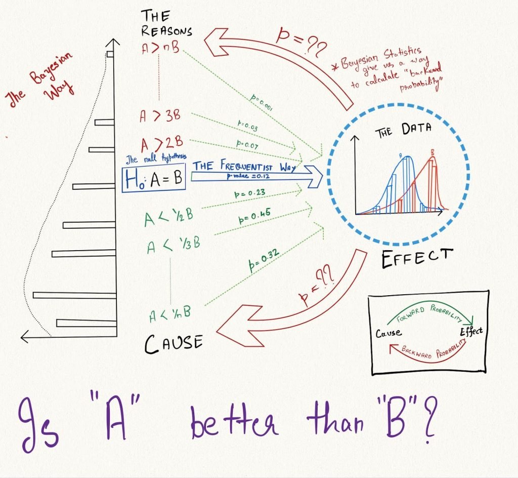
The Frequentists use a null hypothesis which assumes the contrary, there is no effect-size between the control and the variation. The alternate hypothesis says that there is actually a non-zero effect-size between the two. But essentially, the alternate hypothesis is a composite of multiple hypotheses, the effect-size = 1%, effect-size = 2%, effect-size = 3%, and so on (same on the negative side). The Bayesians go through the effort of assuming some probability for each alternate hypothesis. This gives birth to the prior.

The image below shows the difference between the Frequentist Null Hypothesis and the Bayesian Priors. Observe the highlighted p-value and the range of alternate hypotheses below and above the null hypothesis. The vertical distribution on the left represents the probability of each hypothesis which is the prior.

The prior in essence is the entire distribution of possibilities that can be true about the effect-size. Starting with a prior, all variables in a Bayesian algorithm are represented by distributions with some mean and standard deviation. All calculations done are manipulations of these random variables. The final results are also probability distributions called posteriors that give the probabilities of different possibilities.

In summary, think of Bayesians as modern statisticians assisted by advanced computers who simultaneously calculate the probabilities for a range of different cases and then answer which case is the most likely. From an epistemological perspective, Bayesians come with prior beliefs and merge them with the observed evidence to obtain a posterior.

The Bayes Rule vs The T-Distribution

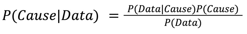
Reverend Thomas Bayes was a statistician and a philosopher who gave the world The Bayes Rule in the 18th century. Before that, there was no way to calculate backward probability (probability of a past cause conditional on a present effect). In the real world, any observed sample can be considered the effect of some latent properties. Hence, in the absence of the Bayes Rule, there was no way to condition on the observed data and estimate the probabilities of the underlying truth. The Bayes Rule is as follows:

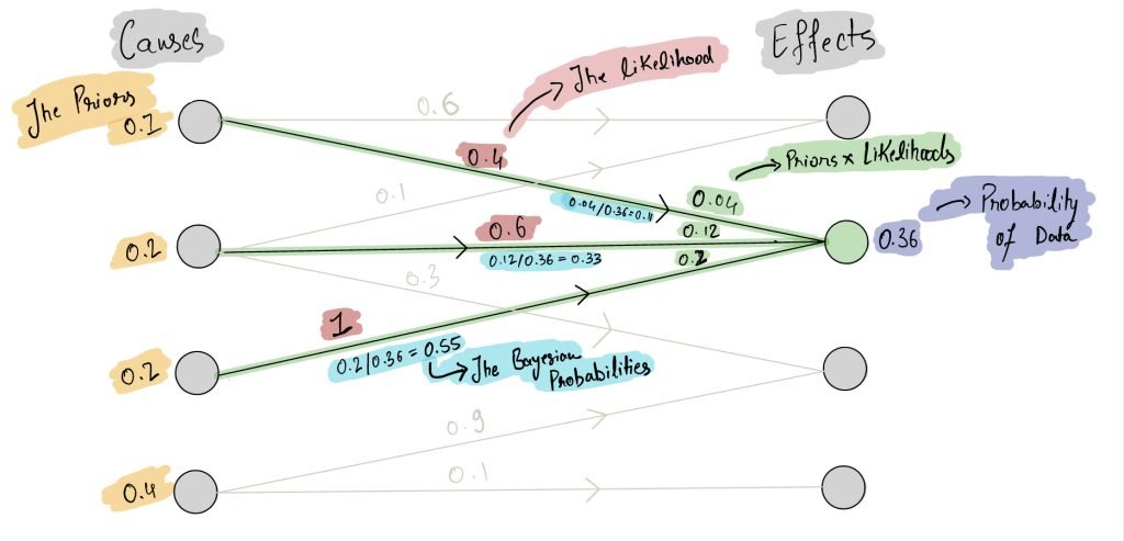
In the diagram below, visually observe how the Bayes Rule works. It first asks for all the causal ways in which the observed outcome can be reached. It then calculates the likelihood of each path (green) by multiplying two probabilities: the prior of the cause (yellow), and the likelihood of the observed effect from that cause (red). The Bayes Rule then calculates the total chance of the observed effect over all paths (purple) and uses it to normalize the forward probabilities (priors x likelihoods). The normalized probabilities are the Bayesian probabilities (light blue) that represent the chance of each cause. Together, these Bayesian probabilities are combined into a posterior distribution over all causes.

In the context of statistical significance, the causes can be considered to be the actual effect size (as depicted in the Is A better than B sketch). The effect is the observed difference in the means of the two samples, one for the control and one for the variation.

The Frequentists do not include the priors in their answer nor do they ever go through the hassle of calculating the Bayesian probabilities. The t-statistic is analogous to the effect as it is a measure of the observed difference. The t-distribution is the likelihood of effect assuming that the null hypothesis is true, P(Data|Cause = Null Hypothesis).

Overall, the only difference between the Frequentists and the Bayesians is the inclusion of priors. Bayes Rule is just a holistic formula that merges the prior and the likelihood into a posterior.

The Posteriors vs The P-value

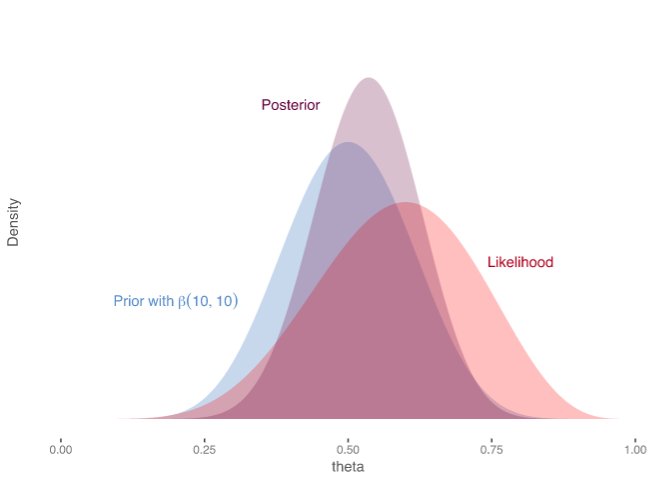
The Frequentists calculate a p-value from the t-distribution which quantifies the chance of observing a difference as extreme as the one observed assuming the null hypothesis was true. The Bayesians on the other hand, calculate the entire set of backward probabilities to define a posterior probability for each possible cause, the effect-size = 1%, effect-size = 2%, effect-size = 3%, and so on. This posterior is interpreted as the updated belief over different causes after observing the data. Note that the posterior always lies between the prior and the likelihood.

The Bayesian posterior is more versatile than the Frequentist p-values as it can be used to answer many more questions. With the posterior, the Bayesians are able to answer complex questions such as:

1. What is the chance that the actual effect-size is in the range <x%,y%>? With the entire posterior available such questions can be directly answered by answering the area under the curve.

2. If a deterioration of 1% in the target metric costs $100, what is the expected loss if the variant is deployed? By using the posterior and further manipulating them with the extra information, Bayesians can calculate the expected value of derived variables as well.

Overall, the posterior distributions once estimated can be powerfully used to calculate different quantities in the entire system. Such a benefit is not available to the Frequentists because they work with the distribution of data and not the distribution of the latent truth. 

Conclusion

An empiricist and his wife are on a drive in the countryside. They come across some sheep and the wife says, “Oh look! Those sheep have been shorn.” 

The empiricist smiles and says, “Yes, on this side.”

Plato and a Platypus Walk Into a Bar by Thomas Cathcart and Daniel Klein

An empiricist is someone who only draws knowledge from his sensory experience. He does not extrapolate that knowledge further. From what was visible to the empiricist on the drive was only one side of the sheep which was towards him, so he drew conclusions only about that side. 

The wife extrapolated the information gathered from her vision to conclude that the sheep were shorn on both sides. The wife could be sure about her conclusions because from prior experience she knows that sheep are usually shorn completely and not just on one side. Had it been a common practice for sheep to be half-shorn, the wife would not have been so sure.

In essence, the debate between the Frequentist and the Bayesian is the same. The Frequentist is like the empiricist because he mixes no prior knowledge when looking at the evidence. The Bayesian is like the wife, he comes with prior knowledge gathered in the past and only looks at evidence in context of the prior information.

But if there is no prior knowledge available to the Bayesian, will he have the same answer as the Frequentist? I will demonstrate the same in the next blog post in this section.