A Critique of the Frequentist and the Bayesian Approach

In 2019, I joined VWO as a young statistician still discovering the deeper problems of randomness. VWO was running Bayesian inference using Monte Carlo Sampling to power the reports for its A/B testing product. In stark contrast to Frequentist methods, millions of samples were being drawn for each calculation requiring multifolds of computational power. The more we explored statistics, the more we were convinced that Bayesian is the way into the future. The only bottleneck was the ability to define the right prior, which was far from easy.

In the search for good priors, Anshul (my teammate) found a method, called bootstrapping, that creates a posterior by randomly resampling from the sample collected (with replacement). It was widely expected that this model-free posterior, entirely based on the sample collected, would represent the true belief about the data-generating process that will boost the accuracy of our systems. But much like Monte Carlo sampling, the method was computationally expensive. We were in dire need of something cheaper that could approximate the results of the bootstrapping method.

Reading through various papers, Anshul brought us a method of approximating posteriors using a normal distribution that very accurately approximated the mean and the standard deviation of the bootstrapped posterior. We had finally stumbled upon a one-line formula that could be calculated in milliseconds. The logical conclusion to our Bayesian statistical engine seemed closer than ever. However, there was one problem.

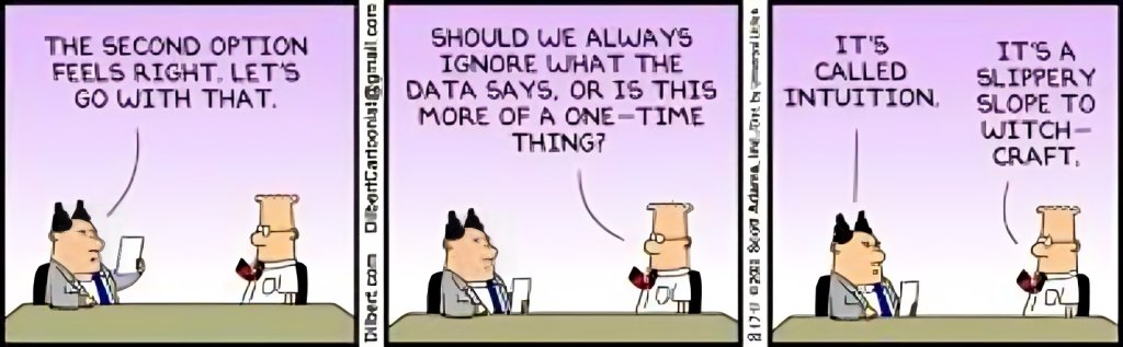
The equation looked eerily similar to the t-statistic. The mean was nothing but the empirical sample mean and the standard deviation was the standard error used by Frequentist methods. Our expedition had taken us through a back door of statistical fascination and led us right to the front door of our unenlightened homes from where we had started. The question we had never dared to ask, now looked at us mischievously as it opened the door for us to digest our failures.

“What is the difference in the final inference from the two methods and why has the entire statistical community not been able to settle the debate for the past 200 years?”

Our redemption into the truth of the Frequentist vs Bayesian debate still awaited us a couple of years ahead, but what lay in front of us was a steep criticism of both methods by opposing statistical factions while the two branches seemed unbelievably intertwined. The criticisms both factions had against each other were legitimate which made the debate even more interesting.

1915 Nobel Laureate William Henry Bragg had once said. “Light behaves like waves on Mondays, Wednesdays and Fridays, like particles on Tuesdays, Thursdays and Saturdays, and like nothing at all on Sundays.” At that moment, we felt the same about Bayesian and Frequentist statistics.

This post is about the unsettled criticisms that the two schools of statistics face, and how they will probably remain unsettled for eternity.

Misinterpreting the P-values

P-values have been notoriously popular in all scientific domains for their misinterpretation. A value that looks very similar to the probability of a study being false, is used as an indicator for the validity of the study, and yet comes with a strong warning to not be interpreted as mere probabilities. Researchers, reporters and science enthusiasts repeatedly published claims based on the p-value that made statisticians facepalm in embarrassment. To be specific, there are three popular ways of misinterpreting the p-values.

1. P-values are the probability that the result is invalid: A layman is justified in summarizing that p-values are the chance that the results of the study are invalid. Note that the result being invalid in reality, is a backward probability question because invalidity is defined by the underlying cause. While p-values are strongly correlated to it, in absolute terms, a p-value of 0.05 can still mean that there is a more than 80% probability that the results are invalid.

2. (1 – P-value) is the chance that the treatment works: Since p-values are not the chance that the results are invalid, it is also wrong to assume that (1 – p-value) is the chance that the treatment worked. Earlier scientific reporters and marketers have often made this mistake. Statistically, one can definitely assume a correlation but again the actual probability is a backward probability that needs an estimation of the prior.

3. (1 – P-value) is the likelihood of the data assuming the alternate hypothesis is true: Those who partially understand p-values often end up making this error. Since p-value represents the likelihood of observing the data assuming the null hypothesis, one often assumes that the inverse might also be true. In other words, if the p-value is 0.03 assuming the null hypothesis, then the p-value assuming the alternative would be 0.97. No, these two probabilities need not sum up to 1 (see the Prosecutor’s fallacy).

The widespread confusion around interpreting p-values is often the pinnacle of Frequentist criticism. It is hard for a layman to understand why p-values defy the logically intuitive corollaries. 

Frequentists have gone to update their methods and calculate a range of p-values corresponding to different alternative hypotheses called confidence curves (similar to the Bayesians), however, there is no way around the twisted meaning of p-values unless we invoke the Bayes Rule. 

Searching for Priors

In essence, priors are nothing but subjective beliefs that represent our past experiences. If you are running an A/B test, and all you had made was a minor change in the color of a small button, then seeing a 30% uplift is surprising. Also, if you drop the prices in half for all your products, and still don’t see a rise in conversion rates, it is surprising as well. Scientific evidence cannot be judged in the absence of what you know. What is surprising is defined by what you already know.

This is the prior that the Bayesians need to really answer the backward probability question, is the variant really better than the control? However, there are three fundamental problems with defining a prior:

1. Priors cannot be estimated from ground truth: There is no way to define priors from ground truth. Someone might say that if you use all your past experiments and study the uplifts you have gotten, then the priors can be estimated. But priors are subjective. Which past tests represent the current test and what the reliability of the uplifts in past tests is a subjective decision and there can be no ground truth to it.

2. Priors are untestable and unfalsifiable: To the best of my knowledge, a prior cannot be tested with evidence collected. Priors can be validated over meta-analysis but only with subjective assumptions on which studies to pick. No evidence can disprove a prior belief without assumptions. Priors do evolve, but slowly and subjectively.

3. Priors are misleading if they are inaccurate: Priors are misleading if they are inaccurately defined. The posterior is always a mix of the prior and the evidence and no matter how much evidence you collect against the prior, the posterior will always be weighed down in a small proportion. Hence, priors do not give an optional one-sided benefit. They can create the need to invest a larger sample size if the evidence contradicts the prior belief.

Owing to the above points, the Frequentists prefer to keep the evidence and the prior beliefs separate. Frequentists refrain from mixing any unfalsifiable and subjective belief into statistical numbers when they look at the data.

Priors might be hard to define, but it does not mean that they do not get taken into account. When you look at the results of a study, you still assess the surprise in the results based on what you know and expect. Priors get included in our judgment if not in numbers.

Conclusion

In summary, I see the Frequentist and the Bayesian in a very deep deadlock. The crux of the problem lies in the interpretations of accuracy. The scientific community essentially cares about the accuracy of the answer given by a statistical method. In other words, what is the chance that the result of an experiment will not replicate if the experiment is run again (false discovery rate)? But in the absence of prior knowledge, this can never be answered accurately. The Frequentist method is closed and complete because it chooses to answer a simpler question, the chance that the experiment will give a winner if there is no underlying effect (false positive rate). It effectively delivers on its guarantees. 

But anyone who has dealt with experimentation for long enough knows that the Bayesian question is the real beast that needs an answer. Bayesian Statistics is then a gamble. Estimate your priors accurately and you can control the false discovery rate. Estimate your priors inaccurately and you might end up requiring more samples to unlearn the inaccurate prior. 

The Frequentist stays away and keeps evidence as evidence. But that does not mean they solve the False Discovery Rate problem either.