The Frequentist Way to Statistical Significance

William Sealy Gosset was a master brewer and a statistician who worked at the Guinness Brewery, Dublin in the early 20th century. Gosset wanted to test the sugar content in the barrels of barley malt extract that was used as a raw material for brewing beers. There was an accepted average and a range of error for the sugar content per barrel. Sugar content was important because it directly determined the alcohol levels of the beer.

But testing all barrels individually was far from viable because if all barrels were used for testing the sugar content, then none would be left for brewing beer. Infact, Gosset wanted to develop a statistical method that would use the least number of barrels and make an estimate about the whole batch.

In 1908, Gosset submitted a paper in a scientific journal, Biometrika with the pseudonym of Student because his employer preferred using a pen name for scientific papers. The rest is history as “Student’s t-test” came to be the standard test of statistical significance used for all scientific studies in the 20th century.

Student’s T-test is interesting to us because it highlights all the structural elements of Frequentist style inference. Gosset’s was not the first Frequentist test of inference and nor was it the last. Different statistical problems have been posed and many different tests have been developed in the Frequentist school of thought. However, all of them have had a similar anatomy: a null hypothesis, a statistic of interest, and a p-value.

In this blog post, we will break open the Frequentist method and understand how it works and why it is designed the way it is. For the purpose of this blog post, let us work with a simple question. We are given two groups of data, the control group and the treatment group and we want to test if the difference between the two groups is statistically significant or not. In other words, we want to test if the treatment had an effect on the target metric or not.

The Null Hypothesis

It is crucial to understand that the question of statistical significance (like most other questions of statistical inference) is fundamentally a backward probability question. Note that we observe the data (the effect) and want to know if the actual data-generating process is different for the two groups or not (the cause). However, for most of history before the invention of computers calculating backward probabilities has been very difficult and required the dependence on a prior. Hence, early statisticians could only rely on calculating the forward probabilities.

Frequentists hence had to take a twisted route of contradiction to determine if two groups are significantly different or not. Frequentists chose to start with the null hypothesis which goes as follows:

“Null Hypothesis: The true mean of the control group and the true mean of the treatment group are actually the same. The difference between the means is 0.”

Note that the null hypothesis always assumes that there is no difference between the two groups and the treatment has not had an effect. Never can it be that a test defines the null hypothesis to be the opposite. There is a reason behind this. If you assume there is no effect, then it is clear that the effect-size is 0. However, if you assume that there is an effect, then you also need to make an assumption on how big the effect-size is.

The Statistic of Interest

After making the assumption, the Frequentist looks for a statistic that can measure the element of surprise the evidence is bringing in. There are a few interesting things to note about the statistic of interest.

1. They are forward probability estimates that refer to some property of the sample collected. For instance, it can be a measure of difference or a measure of disorder.

2. Different tests depending on the properties of the data and the question of inference have different possible statistics. For instance, there are tests of normality that calculate how similar a distribution is to the actual normal distribution.

3. Finally, the statistic is usually accompanied by a distribution which determines the probability of the statistic being as extreme as the observed value. Some example distributions are the Normal, the Chi-square, the F-distribution which are used in different tests.

The distributions themselves are theoretically derived and proven to be an accurate representation of the chosen statistic under some assumptions.

For the purpose of detecting statistical significance, the Frequentists calculate the probability of observing a difference larger than what was observed. I am skipping the derivation of the actual statistic (which is not very difficult, but yes will be boring) and finally showing the encapsulated statistic that the Frequentists finally calculate. 

The t-statistic comes out to be as follows:

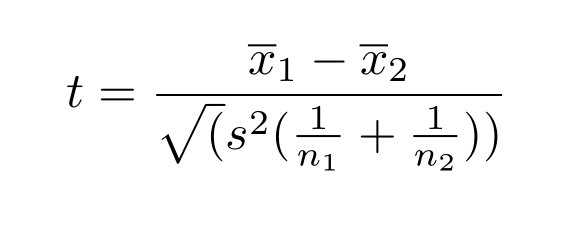
The above represents the t-statistic and once you have the t-statistic you can easily plug it into the standard normal distribution (assuming sample size > 30) and get the chance of observing a difference larger than the one observed (the p-value).

(Observe how the t-statistic is very similar to the relationship behind statistical significance explained here.)

The P-values

P-values are interestingly a source of confusion for many scientists and repeatedly have scientists misinterpreted it or mis-reported it to support their conclusions. The exact definition of the p-value is as follows.

P-value is the chance of observing a result as extreme as observed assuming that there is no difference between the control and the variation.

Frequentists observe the p-values and reject the null hypothesis if the p-value comes below a threshold (usually 0.05 or 0.01). In this way, the Frequentist methodology establishes a difference to be statistically significant if the evidence is too surprising assuming the null hypothesis.

Observe that p-values are forward probabilities and not the probability that the control is equal to the variation. That is probably why statisticians refrain from calling it the probability values. P-values in my opinion are a forward probability answer to a backward probability question.

Conclusion

All Frequentist methodologies of inference follow the same structure as presented above. The only differences that come are in the statistics of interest and the corresponding probability distributions to read the p-values. Frequentist methodologies have dominated science throughout history due to their ease of calculation. However, the Frequentists make a strong assumption that works well in many practical scenarios but is susceptible to risk. The p-values are calculated assuming the null hypothesis, but never assuming the alternate hypotheses. In some scenarios, it is possible that the p-value from the alternate hypotheses is even lower (for instance, in the case of Sally Clark).

Bayesian methods remedy this limitation by assuming a whole range of hypotheses and their associated probabilities (something that they call the priors). In the next blog post, we will explore how the Bayesian approach differs in design from the Frequentist approach.